%reload_ext autoreload
%autoreload 2

import requests
from io import BytesIO
import numpy as np
from PIL import Image
import matplotlib.pyplot as plt
import matplotlib.colors as mcolors

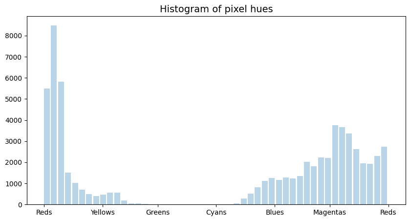
Hues on Color Wheel

On the color wheel, hues form a circle — not a straight line. Reds live near both 0° and 360° (or near 0 and 1 in normalized format).

Naive algorithm may mistakenly think there are two separate groups of reds instead of the true one.

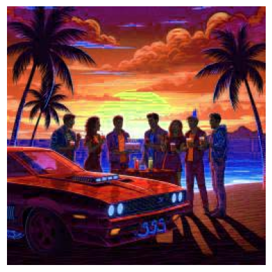
url = "https://github.com/timpyrkov/circleclust/blob/master/tests/image.jpg?raw=true"

# Read image from url (image.jpg from github repository)
response = requests.get(url)
img = Image.open(BytesIO(response.content))

# Show image
plt.imshow(img)
plt.axis('off')
plt.show()

# Convert to RGB array
if img.mode != 'RGB':
    img = img.convert('RGB')
rgb = np.array(img)  / 255

# Convert HSV and extract Hue (H) coordinates on the color wheel
hsv = mcolors.rgb_to_hsv(rgb)
hue = hsv[:, :, 0].flatten()

# Show histogram of hue values in range [0,1)
plt.figure(figsize=(10, 5))
plt.title('Histogram of pixel hues', fontsize=14)
plt.hist(hue, bins=np.linspace(0, 1, 50), width=.017, alpha=.3)

plt.xticks([0.0, 0.17, 0.33, 0.5, 0.67, 0.83, 1.0],
           ["Reds", "Yellows", "Greens", "Cyans", "Blues", "Magentas", "Reds"])

plt.show()

Find Dominant Hues

Detect dominant pixel hues (“Reds” and “Magentas”)

from circleclust import CircleClust

# Initialize and run CircleClust.fit() to find pixel group centroids
cc = CircleClust()
cc.fit(hue, period=1) # Important: provide correct range of data values period!

# Print detected centroids
cc.get_centroids()

{'centroid': array([0.0122247 , 0.85185185]),
 'std': array([0.05099518, 0.12498967])}

# Show detected centroids
cc.show_centroids()

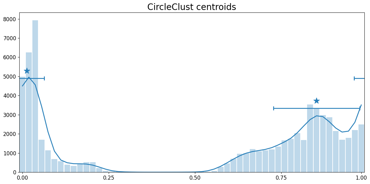
Hue Clusters Size

Note that the “Reds” cluster occupies the area of wrap near Hue = 0. Both pixels close to 0 and close to 1 are attributed to the same single “Reds” cluster.

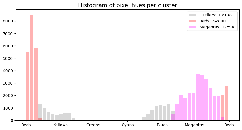
# Run CircleClust.predict() to assign cluster labels
clust_ids = cc.predict(hue, width_scale=1.0)

# Print number of each cluster labels (-1 stands for outliers)
np.unique(clust_ids, return_counts=True)

(array([-1,  0,  1]), array([13138, 24800, 27598]))

# Show histogram of each pixel hue cluster
plt.figure(figsize=(10, 5))
plt.title('Histogram of pixel hues per cluster', fontsize=14)

bins = np.linspace(0, 1, 50)
color = ["grey", "red", "magenta"]
name = ["Outliers", "Reds", "Magentas"]
clist, ccount = np.unique(clust_ids, return_counts=True)
for i, clust_id in enumerate(clist):
    mask = clust_ids == clust_id
    label = f"{name[i]}: {ccount[i]:_}".replace("_", "'")
    plt.hist(hue[mask], bins=bins, width=.017, alpha=.3, color=color[i], label=label)

plt.xticks([0.0, 0.17, 0.33, 0.5, 0.67, 0.83, 1.0],
           ["Reds", "Yellows", "Greens", "Cyans", "Blues", "Magentas", "Reds"])

plt.legend()
plt.show()